Create your Artificial Intelligence (AI) model with Raspberry PI and PyTorch for Image Classification

Last Updated on 6th September 2025 by peppe8o

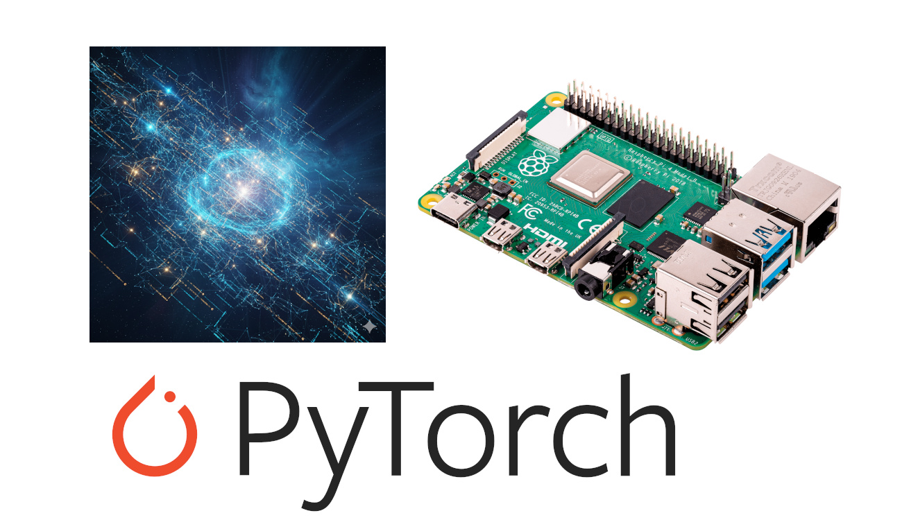
This tutorial will show you how to create a basic Artificial Intelligence (AI) model with a Raspberry PI computer board, using PyTorch. In this tutorial, I will provide you with all the basics to create your own model, while also explaining the neural network that powers it.

About Pytorch

I will not spend many words on it, as this guide is large enough, and I don’t want to waste your time.

Consider that PyTorch is a Python library for machine learning, allowing you to create a neural network and configure it as you want with a few commands. It’s not super easy, as machine learning is a complex topic, but it allows people to get started with an acceptable learning curve.

Our Neural Network

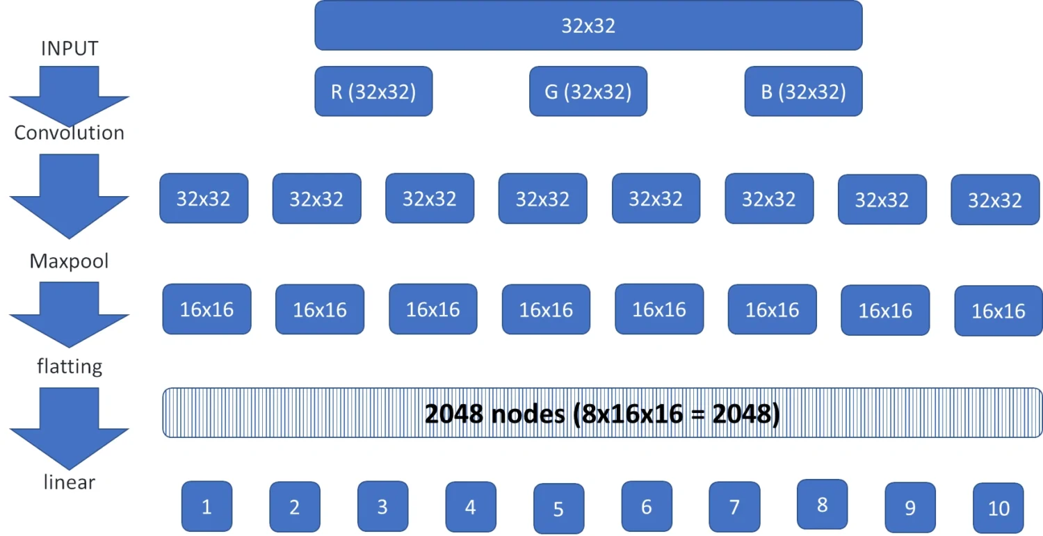
For this test, I’ll set a neural network with 3 layers:

• A convolution layer
• A maxpool layer
• A linear layer

The input will be a 32×32 colour image. The colour image can be considered (and, always transformed) as an RGB (Red, Green, and Blue). This means that we can divide the same image into 3 different images (channels), each one composed only of the red colour, or only the green, or only the blue.

The convolution layer applies a mathematical convolution operation to these 3 input channels, producing as output 8 channels.

The Maxpool layer gets as input the 8 channels from the previous layer and practically resizes them into 8 channels with a lower size (16×16). During this resize, the Maxpool function outputs only the most important pixels from the original channel.

Before reaching the final layer, a “flatting” operation will convert all of these 16×16 channels into a “single string” by using each row of every channel. So, from 8 channels with 16×16 size, we’ll have 8 x 16 x 16 = 2048 single nodes.

With the “flatting” operation done, the last linear layer will be able to convert the input nodes into 10 outputs.

The whole neural network can be simplified as in the following picture:

In order to work, every layer must use specific parameters for the convolution and linear operations: weights and biases. At the beginning of any train session, all of these parameters are set with default values.

Forward and Backwards Propagation

During the training process, the neural network will change them according to the machine learning goal: the “forward” process (from top to bottom in the picture) will try to evaluate an image; if the result is wrong, the “backwards” process will try to optimise all the parameters of the chain (from bottom to top).

These parameters are those we’ll save as a model at the end of the process.

If you want to learn more about neural networks, I strongly suggest reading the book by Melanie Mitchell: “Artificial Intelligence A Guide for Thinking Humans” I found it really useful for my knowledge about Artificial Intelligence, and she explains in a very clear way how it works. You can search it in your local Amazon store with this link.

What We Need

As usual, I suggest adding from now to your favourite e-commerce shopping cart all the needed hardware, so that at the end you will be able to evaluate overall costs and decide if to continue with the project or remove them from the shopping cart. So, hardware will be only:

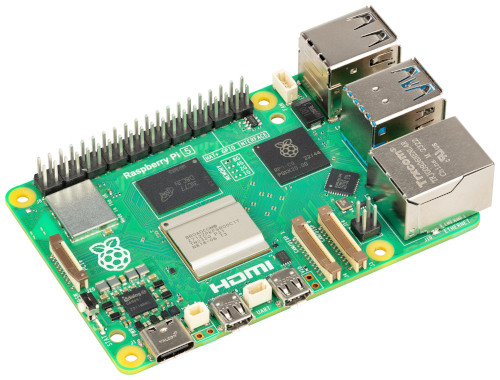
• Raspberry PI Computer Board (including proper power supply or using a smartphone micro USB charger with at least 3A)
• high-speed micro SD card (at least 16 GB, at least class 10)

For this tutorial, I will use my Raspberry PI 5 Model B with 8GB of RAM. If you use a Raspberry PI model with a lower amount of RAM, I strongly suggest increasing the Raspberry PI SWAP memory with the linked tutorial.

Step-by-step Procedure

Prepare the Raspberry PI Operating System

The first step is installing the Raspberry PI OS Lite (I suggest the 64-bit version, for boards supporting it) to get a fast and light operating system (headless). If you need a desktop environment, you can also use the Raspberry PI OS Desktop, in this case working from its terminal app. Please find the differences between the 2 OS versions in my Raspberry PI OS Lite vs Desktop article. For low RAM Raspberry PI computer models, the Lite OS is strongly suggested.

For this test, I will use a Raspberry PI OS Lite headless installation. However, a Desktop installation also works by using the terminal.

Please make sure that your OS is up to date. From your terminal, use the following command:

sudo apt update -y && sudo apt full-upgrade -y

We also need to install the PIP package manager:

sudo apt install python3-pip -y

Install PyTorch on Raspberry PI

We also need to create a Python Virtual Environment in Raspberry PI (with the complete guide from the link). Please refer to it about how to use and how to activate/deactivate it (you need to activate the virtual environment every time you logout from the Raspberry PI). Below are the short commands:

python -m venv my_ai
source ./my_ai/bin/activate

In the following part of the tutorial, I will suppose that you’ll leave this virtual environment active.

Now, we can proceed by installing the required packages. With PIP, you can perform this task from the following terminal command:

pip install torch torchvision

Train the AI model with Raspberry PI with CIFAR-10

We’ll use a free dataset to train this model: the CIFAR-10. It includes 60,000 colour images (32 pixels x 32 pixels). From this set, 50,000 are for training and 10,000 are for testing the training process. The CIFAR-10 dataset includes 10 image classes: airplane, automobile, bird, cat, deer, dog, frog, horse, ship, and truck. So, a model trained with this dataset will be able to classify only these classes of objects.

You can get the complete code from my download area directly in your Raspberry PI storage with the following command:

wget https://peppe8o.com/download/python/pytorch/train_cifar10.py

The following paragraphs will explain the code line by line.

Importing the Required Packages and Datasets

At the beginning, we import the needed Python libraries:

import torch
import torchvision
import torchvision.transforms as transforms
import torch.nn as nn
import torch.nn.functional as F
import torch.optim as optim

After this, we set up the transform function. For each imported image from the dataset, this will convert the image into a tensor and then normalise each channel (red, green, and blue) according to its “mean value” (the first (0.5, 0.5, 0.5) set) and a standard deviation (the second (0.5, 0.5, 0.5) set). This operation is vital, both in the training process as in the prediction process, to get our AI model working always on images calibrated around the same values.

transform = transforms.Compose(
    [transforms.ToTensor(),
     transforms.Normalize((0.5, 0.5, 0.5), (0.5, 0.5, 0.5))])

Instead of keeping all the 50,000 train images in a single, big, train step, we divide them into smaller batches. In this way it will be easier for our Raspberry PI to deal with the processing job. The same concept will be applied also to the testing step. For this reason, we define the batch_size variable:

batch_size = 64

The following lines will download the train and the test datasets to our Raspberry PI’s storage, inside a “.data” hidden folder in the current path. The dataloader function will organise them into an iterable object, making it easier for the script to access them during the training and test steps:

trainset = torchvision.datasets.CIFAR10(root='./data', train=True, download=True, transform=transform)
trainloader = torch.utils.data.DataLoader(trainset, batch_size=batch_size, shuffle=True, num_workers=2)

testset = torchvision.datasets.CIFAR10(root='./data', train=False, download=True, transform=transform)
testloader = torch.utils.data.DataLoader(testset, batch_size=batch_size, shuffle=False, num_workers=2)

Defining the Neural Network

Now, we can define our neural network. The following class identifies the layers in the __init__ function, while the forward function will detail how the data will flow in our network. It is important to note that the Conv2d (the convolution function which defines the related layer) has 3 input channels and 8 output channels, while defining the used filter (kernel size) into a 3×3 window. The Linear funcion will convert 8 channels, each one with 16×16 size, into a 2,048 outputs.

The ReLU (Rectified Linear Unit) function, also known as “activation function”, parses all the records that are given as input and zeroes the negative values (keeping the positive with their value). In this way, the negative values will not impact the calculations of the model, as these values can be considered without interest:

class NeuralNet(nn.Module):
    def __init__(self):
        super().__init__()
        self.conv1 = nn.Conv2d(3, 8, kernel_size=3, padding=1)
        self.pool = nn.MaxPool2d(2, 2)
        self.fc1 = nn.Linear(8 * 16 * 16, 10)

    def forward(self, x):
        # Layer 1
        x = self.conv1(x)
        x = F.relu(x)
        # Layer 2
        x = self.pool(x)
        # Layer 3
        x = torch.flatten(x, 1)
        x = self.fc1(x)
        x = F.relu(x)
        return x

Now, we can initialise our neural network. A print statement will allow you to see it in your terminal when the script is running:

net = NeuralNet()
print(net)

The next two important lines will define the function which calculates the loss at every estimation, as well as the optimize function (how and how fast the network parameters should change in case of errors detected during the training process):

loss_fn = nn.CrossEntropyLoss()
optimizer = optim.SGD(net.parameters(), lr=0.001)

The Training Process

This part of the process can be enclosed in a custom function.

At the beginning of this function, we define the “size” variable just to know how many samples we have in our dataset for stats at the end of the training process. Then, we put the model into train mode:

def train(dataloader, model, loss_fn, optimizer):
    size = len(dataloader.dataset)
    model.train()

A loop starts now, iterating over the images obtained from the dataloader in batches. The first step during the training is just predicting the current image and calculating the loss (if any):

    for batch, (inputs, labels) in enumerate(dataloader):
        prediction = model(inputs)
        loss = loss_fn(prediction, labels)

Once we know the loss, we can activate the back-propagation to optimise the model’s parameters according to the registered loss:

        loss.backward()
        optimizer.step()
        optimizer.zero_grad()

When the batch is complete, we can calculate the total value of the loss for this batch and print it as stats in the terminal, so that you can clearly see how the training is progressing:

        if batch % 100 == 0:
            loss, current = loss.item(), (batch + 1) * len(inputs)
            print(f"loss: {loss:>7f}  [{current:>5d}/{size:>5d}]")

The Testing Process

After you train your Artificial Intelligence model on a Raspberry PI, you need to check if it’s reliable before using it. This is the goal fr the testing process. It must give us statistics on the accuracy of our model.

At the beginning of this new function, we need to get the size of the test dataset and to set the number of batches as follows, for statistics purposes:

def test(dataloader, model, loss_fn):
    size = len(dataloader.dataset)
    num_batches = len(dataloader)

After this, we put the model into the evaluation model. We also initialise the value of loss and correct predictions:

    model.eval()
    test_loss, correct = 0, 0

The following lines will pop an image at once from the dataset. It tries to predict the label. The argmax(1) in our prediction will allow you to get only the first label predicted from the model.

After this, if the predicted value is wrong, the test_loss will be updated with the distance to the correct label. In case of a correct prediction, this function will return a zero, and the following line will update the correct counter.

    with torch.no_grad():
        for inputs, labels in dataloader:
            prediction = model(inputs)
            test_loss += loss_fn(prediction, labels).item()
            correct += (prediction.argmax(1) == labels).type(torch.float).sum().item()

The final rows will prepare the resulting stats about how the model performed in the whole dataset, and will print it:

    test_loss /= num_batches
    correct /= size
    print(f"Test Error: \n Accuracy: {(100*correct):>0.1f}%, Avg loss: {test_loss:>8f} \n")

Running the Training Epochs

AI model tuning usually repeats the training and testing steps several times on the same dataset. This allows the model to improve its neural network parameters, even if it is running on the same dataset. The number of new iterations on the same dataset is referred to as an epoch. Usually, AI models are trained in something between 20 and 50 epochs.

Even if the more epochs you use, the more your model will be reliable, increasing this number too much will make the model “overfitted”. This means that the model has been trained too much on the same dataset and will perform with bad results once you use it with new images not included in it.

At the beginning of the final part of our script, we set the number of epochs into a variable, so that you can easily identify it if you want to change this number:

epochs = 5

With the custom functions previously created, the main part of our script will be extremely simplified.

For each epoch, after printing a short message about the current epoch number, it will train the AI model on the train dataset and test it. This job is made with the following 3 lines:

for t in range(epochs):
    print(f"Epoch {t+1}\n-------------------------------")
    train(trainloader, net, loss_fn, optimizer)
    test(testloader, net, loss_fn)

After the training is finished, a message will advise us about the end of the process:

print('Finished Training')

Before closing the script, we save our AI model in the current path with the name “my_model.pth”:

PATH = './my_model.pth'
torch.save(net.state_dict(), PATH)

Run the Artificial Intelligence Training on Raspberry PI

Now, you can train this AI model with the following terminal command (with the Python virtual environment active):

python train_cifar10.py

You will see your Neural Network structure printed on the terminal:

NeuralNet(
  (conv1): Conv2d(3, 8, kernel_size=(3, 3), stride=(1, 1), padding=(1, 1))
  (pool): MaxPool2d(kernel_size=2, stride=2, padding=0, dilation=1, ceil_mode=False)
  (fc1): Linear(in_features=2048, out_features=10, bias=True)
)

Then the script will show you the progress for the training process, as described in the previous paragraphs:

Epoch 1
-------------------------------
loss: 2.306931  [   64/50000]
loss: 2.268831  [ 6464/50000]
loss: 2.249069  [12864/50000]
loss: 2.211246  [19264/50000]
loss: 2.273102  [25664/50000]
loss: 2.174660  [32064/50000]
loss: 2.259000  [38464/50000]
loss: 2.303093  [44864/50000]
Test Error:
 Accuracy: 26.3%, Avg loss: 2.160020

Epoch 2
-------------------------------
loss: 2.206101  [   64/50000]
loss: 2.189285  [ 6464/50000]
loss: 2.107840  [12864/50000]
(...)

Final Thoughts

The model trained with this example script will give you a low accuracy level. To make it more accurate, please increase the number of epochs: it will take more time, but you will see the accuracy level increase epoch by epoch.

You can also change the structure of your neural network by increasing the number of layers and adding more nodes. For this scope, you must pay attention to keep a consistent structure: the number of outputs of each layer should always be compliant with the number of inputs on the following layer.

What’s Next

In my next tutorial for this series, I will show how to use this model. The following articles will also show you how to customise your dataset. Subscribe to my newsletter to stay tuned!

If you are interested in more Raspberry PI projects (both with Lite and Desktop OS), take a look at my Raspberry PI Tutorials.

Enjoy!