
Last Updated on 27th June 2026 by peppe8o
This tutorial will show you how to use a Raspberry PI for Stock Market monitoring and analysis with a few Python code lines and for free. It will show you how to get professional tools into your Raspberry PI computer board, without the need for expensive services.
In this guide, I will use pandas DataFrame to store the stock values, creating a dashboard with Dash and Plotly. Then I’ll add moving average lines. After these tests, I will also provide you the performance checks to evaluate what is the computing load.
This Tutorial Focus
This tutorial will not cover strategies and how to earn money with the Stock Market exchanges, as this isn’t the goal of the article, because it is really risky (and you must know the risks before starting), and because the web is plenty of people and websites that do this as job. But you will get all the tools for monitoring and automating your trading signals, so this can be useful also for professional traders wishing to add monitoring tools at a very cheap cost, only for the Raspberry PI computer board.
Before starting, please note that financial stocks are identified by a symbol representing both the stock and the exchange market where it is traded. For example, Intesa San Paolo is an Italian bank traded in the Milan Exchange with the symbol “ISP.MI”, where the part after the dot identifies the exchange. I will assume here that you will select your stocks with this symbol notation.
What you will build
The final result is a small web app, based only on Python, that:
- reads stock data from a pandas DataFrame,
- shows an interactive candlestick chart,
- adds one or more tool lines,
- runs on your Raspberry PI and can be opened remotely in a browser.
This approach is beginner-friendly because the chart logic stays short, while the user still gets zoom, hover, and toolbar controls in the browser through Plotly.
What We Need
As usual, I suggest adding from now to your favourite e-commerce shopping cart all the needed hardware, so that at the end you will be able to evaluate overall costs and decide if to continue with the project or remove them from the shopping cart. So, hardware will be only:
- Raspberry PI Computer Board (including proper power supply or using a smartphone micro USB charger with at least 3A)
- high speed micro SD card (at least 16 GB, at least class 10)
I’ve tested this tutorial with my Raspberry PI 5 model B, but it should work well even on a cheap Raspberry PI Zero 2 W computer board.
Step-by-Step Procedure
Step 1. Prepare the Operating System
The first step is to install the Raspberry PI OS Lite to get a fast and lightweight operating system (headless). If you need a desktop environment, you can also use the Raspberry PI OS Desktop, in which case you will work from its terminal app. Please find the differences between the 2 OS versions in my Raspberry PI OS Lite vs Desktop article.
Please make sure that your Operating System is up to date. From your terminal, use the following command:
sudo apt update -y && sudo apt full-upgrade -yStep 2. Install the required Packages
We need some packages to get our program working. The packages require pip:
sudo apt install python3-pipWith the latest releases, we need to use a Python Virtual Environment to install packages via pip. The provided link will give you a deep explanation on how they work.
Please create a virtual environment (I will name it as “stock_dash”, but you can name the environment as you prefer):
python3 -m venv stock_dashActivate it. Please remember that you must activate the virtual environment every time you want to use the app. Moreover, in the following command change “stock_dash” with the name you gave to your virtual environment, if you used a different one):
source stock_dash/bin/activateThe virtual environment will be active as you see its name at the beginning of your prompt:
(stock_dash) pi@raspberry:~ $Now, we can install the required packages:
pip3 install pandas yfinance TA-Lib dashStep 3. Download on Raspberry PI the Stock Market Data
Let’s create our script. From the terminal:
nano stock.pyPlease fill the file with the following content:
#From peppe8o.com
import yfinance as yf
import pandas as pd

history_to_download = "4y"
s = "ISP.MI"

stock_ticker = yf.Ticker(s)
df = stock_ticker.history(period=history_to_download)

print(df)
Save and close the file.
In this script:
- After the small comment line including a reference to my blog (the first line), we import the required packages.
- Then, we set the amount of history data we want to download (in this example, 4y means 4 years).
- The
svariable stores the stock name. In this case, I will download the quotes about the Intesa San Paolo from the Milan stock exchange. - Then, we create a Ticker object, which we’ll use to download the data.
- The
df = stock_ticker.history(...)line will download them and store the data in a pandas dataframe. - The last command will just print this dataframe.
Please run this simple script with the following command:
python stock.pyIt will give you a result similar to the following:
(stock_dash) pi@raspberry:~ $ python stock.py
                               Open      High       Low     Close     Volume  Dividends  Stock Splits
Date
2022-06-27 00:00:00+02:00  1.404778  1.426671  1.377777  1.381718  147678067        0.0           0.0
2022-06-28 00:00:00+02:00  1.390037  1.412659  1.385513  1.385513  114640001        0.0           0.0
2022-06-29 00:00:00+02:00  1.370479  1.384929  1.361722  1.369020   92133124        0.0           0.0
2022-06-30 00:00:00+02:00  1.344208  1.347127  1.284077  1.298964  193939309        0.0           0.0
2022-07-01 00:00:00+02:00  1.284223  1.308742  1.268752  1.289915  149502743        0.0           0.0
...                             ...       ...       ...       ...        ...        ...           ...
2026-06-22 00:00:00+02:00  6.172000  6.234000  6.120000  6.234000   47338191        0.0           0.0
2026-06-23 00:00:00+02:00  6.185000  6.226000  6.107000  6.131000   55597443        0.0           0.0
2026-06-24 00:00:00+02:00  6.133000  6.146000  6.077000  6.093000   40627685        0.0           0.0
2026-06-25 00:00:00+02:00  6.100000  6.109000  6.003000  6.030000   59515068        0.0           0.0
2026-06-26 00:00:00+02:00  5.993000  6.001000  5.900000  5.952000   51494539        0.0           0.0

[1015 rows x 7 columns]
As you can see, the dataframe includes all the main data required for a stock analisys.
Step 4. Create the candlestick chart
We’ll start with the smallest useful app, just showing the downloaded values.
Please open the previsous script for editing:
nano stock.pyYou can remove the last line (print(df)) and append the following lines:
# Import the chart packages
from dash import Dash, dcc, html
import plotly.graph_objects as go

# Create the figure
fig = go.Figure(data=[go.Candlestick(
    x=df.index,
    open=df["Open"],
    high=df["High"],
    low=df["Low"],
    close=df["Close"]
)])

# Figure settings
fig.update_layout(xaxis_rangeslider_visible=False)
fig.update_yaxes(fixedrange=False)
fig.update_layout(height=700)

# Initialise and run the Dash app
app = Dash(__name__)
app.layout = html.Div([
    html.H1(s + " stock chart"),
    dcc.Graph(figure=fig)
])

# Starts the app server
if __name__ == "__main__":
    app.run(host="0.0.0.0", port=8050, debug=True)
Save and close.
In this block:
- We import the additional packages we need to create the chart app
- The
fig = go.Figure(...)creates a Plotly figure containing one candlestick chart built from your DataFrame - The
fig.update_xxxconfigure some settings to the figure to manage the chart axes and the chart height - The
appblock creates our web app and adds the chart in it - The last block initialises the web server
Now, you can run this script with the same terminal command:
python stock.pyFrom the terminal side, you will just see a debug info:
(stock_dash) pi@raspberry:~ $ python stock.py
Dash is running on http://0.0.0.0:8050/

 * Serving Flask app 'stock'
 * Debug mode: on
From a browser (on a remote PC or in the same Raspberry PI OS if you use the Desktop version, please use the Raspberry PI’s IP address and port 8050 (http://192.168.1.218:8050/ in my case) to reach the web app. You will see something like the following:
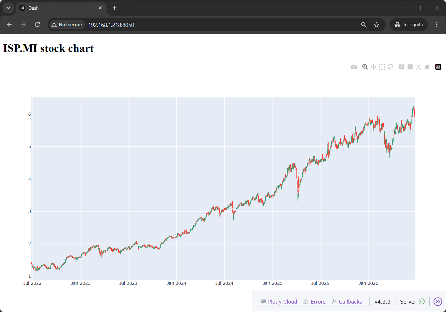
By moving the mouse on the chart, you will see the chart tools appearing on the top-right side. By default, you will have the zoom tool, which is a cross pointer enabling you to select any area of the chart to zoom it. Here you can also select other visualization tools.
At any time, you can stop the server app with the CTRL+C on the terminal.
Step 5. Add SMA (Simple Moving Average) Lines
We’ll use the TA-Lib package to add SMA lines (as well as any other indicators supported by the TA-Lib package).
Let’s open the file again:
nano stock.pyPlease add the following content before the app definition blocks.
# Import the indicators package
import talib

# Add the lines to the DataFrame
df["SMA10"] = talib.SMA(df["Close"], timeperiod=10)
df["SMA30"] = talib.SMA(df["Close"], timeperiod=30)

# Add the lines to the chart
fig.add_trace(go.Scatter(
    x=df.index,
    y=df["SMA10"],
    mode="lines",
    name="SMA10",
    line=dict(color="orange", width=2, dash="solid")
))

fig.add_trace(go.Scatter(
    x=df.index,
    y=df["SMA30"],
    mode="lines",
    name="SMA30",
    line=dict(color="blue", width=2, dash="solid")
))
Save and close.
Here’s the block explanation:
- The first block imports the required packages
- The second block uses the
talib.SMA(...)function from the TA-Lib library to calculate SMA values and appends them to the same dataframe where the stock values are stored - With the last block, the
fig.add_trace(...)lines add the created indicators to the chart. In these lines, I also added some options (not mandatory) to allow you customising the appearence of the lines.
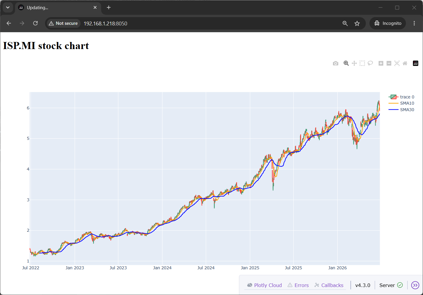
Please run again this script:
python stock.pyFrom the browser, you will see the lines included in the chart:
Tips and Tricks
Add Multiple SMA Lines
When adding multiple indicators with different periods, you may find ineffective copying multiple fig.add_trace(...) blocks. In this case, you may use the following function instead:
for n, color in [(10, "orange"), (20, "deepskyblue"), (50, "limegreen")]:
    df[f"SMA{n}"] = df["Close"].rolling(n).mean()
    fig.add_trace(go.Scatter(
        x=df.index,
        y=df[f"SMA{n}"],
        mode="lines",
        name=f"SMA{n}",
        line=dict(color=color, width=2)
    ))
Make the Chart Taller
If the chart area feels too small, increase the figure or graph height. Plotly supports fig.update_layout(height=…) (as seen in my script), and Dash also supports a CSS-style height on dcc.Graph(…):
dcc.Graph(
    figure=fig,
    style={"height": "700px"},
    config={"scrollZoom": True}
)
You can use the one or the other at your choise.
Zoom Behavior
Candlestick charts in Plotly can zoom well on the x-axis, but the y-axis does not always rescale automatically to only the visible candles. This is a known behavior discussed in Plotly community threads.
The fig.update_yaxes(fixedrange=False) fixed the issue for me, but there may be cases where it doesn’t work well. In these cases, the solution may be restricting the data history to download.
Automating Raspberry PI Stock Market Signals
Now, you have your Stock quotes and Technical Indicators in your Raspberry PI. Besides showing the chart, the question is: how can this help me?
The answer is that Raspberry PI computer boards are very low power consumption devices, so you can keep them powered on every day without risking high energy bills. Moreover, you can configure them to run specific tasks to run at a specified frequency. Using a Cron Job, you can download the stock data and compare the price value every day, then send email warnings to your email address at your signals trigger.
The process of sending emails with a standard Python script and a Cron job is explained in my Send Email from Raspberry PI with Python tutorial. Keep the tutorial and mix it with the p8o-finance-no-chart.py script in order to reach your goal.
Performances on Raspberry PI 5 Model B (8GB)
To measure the performances both in CPU, RAM, and time elapsed, I will use the time package:
sudo apt install time -yWith this, you can measure your performances with the following terminal command:
/usr/bin/time -v python stock.pyHere are my perfomances.
Board: Raspberry PI 5 Model B (8 GB).
Download data:
| CPU | 74 % (only 1 core out of 4) |
| RAM | 103 MB |
| Time elapsed | ~1 second |
Dash app running with a simple chart:
| CPU | 24% (only 1 core out of 4) |
| RAM | 142 MB |
| Time elapsed (Dash App boot) | 2 seconds |
As you can see, this script uses a very low amount of resources, making it perfect for a Raspberry PI stock market monitor and analisys tool.
Next Steps
Interested in more projects with your RPI? Try to look at my Raspberry PI computer tutorial pages.
Enjoy!

Open source and Raspberry PI lover, writes tutorials for beginners since 2019. He's an ICT expert, with a strong experience in supporting medium to big companies and public administrations to manage their ICT infrastructures. He's supporting the Italian public administration in digital transformation projects.
![]()
![]()
![]()
![]()
![]()
![]()
![]()


I am using clean install of Debian 13.5 Trixie. Fully upgraded. I am trying to install your stock tracking and charting software. I got to second line of download instructions. sudo apt install python3-pip worked fine. pip3 install pandas mplfinance pandas_ta failed: externally-managed-environment error.
It suggested “try install python3-xyz where xyz is package name.” sudo apt install python3-pandas worked. mplfinance and pandas_ta did not. Any thoughts?
Hi Ric. With newest Python versions you must use virtual environments. I’ll update this tutorial soon (today or tomorrow) as testing it again there are some changes to make, and I want to show easier tools. Stay tuned!
Hi Ric, I just published a new tutorial. Please let me know if this works and you feedback